Fitting distributions to data with paramnormal.¶

In addition to explicitly creating distributions from known parameters, paramnormal.[dist].fit provides a similar, interface to scipy.stats maximum-likelihood estimatation methods.

Again, we’ll demonstrate with a lognormal distribution and compare parameter estimatation with scipy.

%matplotlib inline

import warnings
warnings.simplefilter('ignore')

import numpy as np
import matplotlib.pyplot as plt
import seaborn

import paramnormal

clean_bkgd = {'axes.facecolor':'none', 'figure.facecolor':'none'}
seaborn.set(style='ticks', rc=clean_bkgd)

Let’s start by generating a reasonably-sized random dataset and plotting a histogram.

The primary method of creating a distribution from named parameters is shown below.

The call to paramnormal.lognornal translates the parameter to be compatible with scipy. We then chain a call to the rvs (random variates) method of the returned scipy distribution.

np.random.seed(0)
x = paramnormal.lognormal(mu=1.75, sigma=0.75).rvs(370)

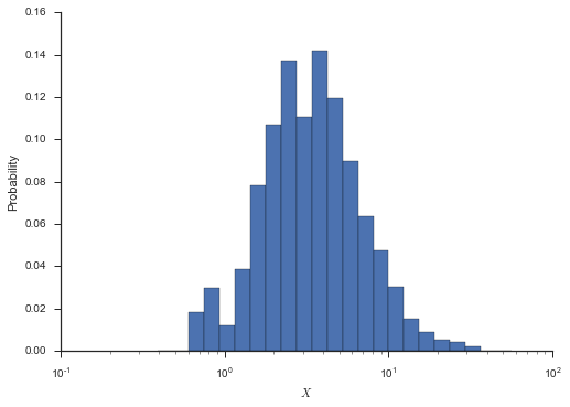
Here’s a histogram to illustrate the distribution.

bins = np.logspace(-0.5, 1.75, num=25)
fig, ax = plt.subplots()
_ = ax.hist(x, bins=bins, normed=True)
ax.set_xscale('log')
ax.set_xlabel('$X$')
ax.set_ylabel('Probability')
seaborn.despine()
fig

Pretending for a moment that we didn’t generate this dataset with explicit distribution parameters, how would we go about estimating them?

Scipy provides a maximum-likelihood estimation for estimating parameters:

from scipy import stats
print(stats.lognorm.fit(x))

(0.77953564806411113, 0.23350251237627717, 5.3711822451406039)

Unfortunately those parameters don’t really make any sense based on what we know about our articifical dataset.

That’s where paramnormal comes in:

params = paramnormal.lognormal.fit(x)
print(params)

params(mu=1.7370786294627456, sigma=0.73827268519387368, offset=0)

This matches well with our understanding of the distribution.

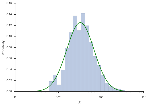
The returned params variable is a namedtuple that we can easily use to create a distribution via the .from_params methods. From there, we can create a nice plot of the probability distribution function with our histogram.

dist = paramnormal.lognormal.from_params(params)

# theoretical PDF
x_hat = np.logspace(-0.5, 1.75, num=100)
y_hat = dist.pdf(x_hat)

bins = np.logspace(-0.5, 1.75, num=25)
fig, ax = plt.subplots()
_ = ax.hist(x, bins=bins, normed=True, alpha=0.375)
ax.plot(x_hat, y_hat, zorder=2, color='g')
ax.set_xscale('log')
ax.set_xlabel('$X$')
ax.set_ylabel('Probability')
seaborn.despine()

params = paramnormal.lognormal.fit(x)
print(params)

params(mu=1.7370786294627456, sigma=0.73827268519387368, offset=0)

paramnormal.lognormal(mu=1.75, sigma=0.75, offset=0)

<scipy.stats._distn_infrastructure.rv_frozen at 0x111614f98>

paramnormal.lognormal.from_params(params)

<scipy.stats._distn_infrastructure.rv_frozen at 0x1116142e8>