Paramnormal Activity¶

Perhaps the most convenient way to access the functionality of paramnormal is through the activity module.

Random number generation, distribution fitting, and basic plotting are exposed through activity.

%matplotlib inline

import warnings
warnings.simplefilter('ignore')

from numpy.random import seed
from scipy import stats
from matplotlib import pyplot
import seaborn

import paramnormal

clean_bkgd = {'axes.facecolor':'none', 'figure.facecolor':'none'}
seaborn.set(style='ticks', rc=clean_bkgd)

Random number generation¶

Through the top-level API, you could do the following to generate lognormal random numbers.

seed(0)
paramnormal.lognormal(mu=0.75, sigma=1.25).rvs(5)

array([ 19.20297918,   3.49102891,   7.19526003,  34.85220823,  21.85538813])

What’s happening here is that paramnormal.lognormal(mu=0.75, sigma=1.25) translates the arguments, passes them to scipy.stats.lognorm, and returns scipy’s distribution object. Then we call the rvs method of that object to generate five random numbers in an array.

Through the activity API, that equivalent to:

seed(0)
paramnormal.activity.random('lognormal', mu=0.75, sigma=1.25, shape=5)

array([ 19.20297918,   3.49102891,   7.19526003,  34.85220823,  21.85538813])

And of course, Greek letters are still supported.

seed(0)
paramnormal.activity.random('lognormal', μ=0.75, σ=1.25, shape=5)

array([ 19.20297918,   3.49102891,   7.19526003,  34.85220823,  21.85538813])

Lastly, you can reuse an already full-specified distribution and the shape parameter can take a tuple to return N-dimensional arrays.

seed(0)
my_dist = paramnormal.lognormal(μ=0.75, σ=1.25)
paramnormal.activity.random(my_dist, shape=(2, 4))

array([[ 19.20297918,   3.49102891,   7.19526003,  34.85220823],
       [ 21.85538813,   0.62400472,   6.94214304,   1.75207971]])

Fitting distributions¶

Fitting distributions to data follows a similar pattern.

data = paramnormal.activity.random('beta', α=3, β=2, shape=37)
paramnormal.activity.fit('beta', data)

params(alpha=2.609817838242197, beta=1.9104280289172266, loc=0, scale=1)

Equivalent command to perform the same fits in raw scipy is shown below:

# constrained loc and scale
stats.beta.fit(data, floc=0, fscale=1)

(2.609817838242197, 1.9104280289172266, 0, 1)

You can still fix the primary parameters and unconstrain the defaults.

paramnormal.activity.fit('beta', data, β=2, loc=None)

params(alpha=2.7441640478582361, beta=2, loc=-0.0031375474001911555, scale=1)

And again in raw scipy:

# constrained beta and scale, unconstrained loc
stats.beta.fit(data, f1=2, fscale=1)

(2.7441640478582361, 2, -0.0031375474001911555, 1)

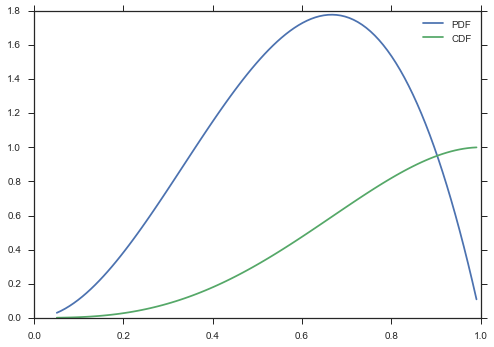
Plotting¶

There is very limited plotting functionality built into paramnormal. The probability distribution function (PDF) is plotted by default, but any other method of the distributions can be plotted by specifying the which parameters.

ax = paramnormal.activity.plot('beta', α=3, β=2)
paramnormal.activity.plot('beta', α=3, β=2, ax=ax, which='CDF')
ax.legend()

<matplotlib.legend.Legend at 0x10f0a1f98>

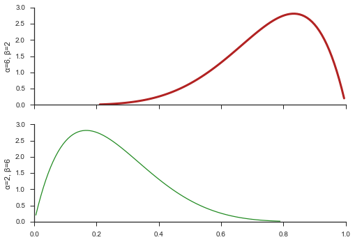
You can plot on an existing figure through the ax argument and control the line style through line_opts.

fig, (ax, ax2) = pyplot.subplots(nrows=2, sharex=True, sharey=True)
paramnormal.activity.plot('beta', α=6, β=2, ax=ax, line_opts=dict(color='firebrick', lw=3))
paramnormal.activity.plot('beta', α=2, β=6, ax=ax2, line_opts=dict(color='forestgreen', lw=1.25))
ax.set_ylabel('α=6, β=2')
ax2.set_ylabel('α=2, β=6')
seaborn.despine(fig)

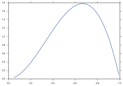
Of course, you can create a fully-specified distribtion and omit the distribution parameters.

beta = paramnormal.beta(α=3, β=2)
ax = paramnormal.activity.plot(beta)

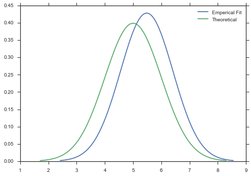
And finally, you can pass an array of data and an unfrozen distribution, and a new distribution will be fit to your data.

data = paramnormal.activity.random('beta', α=2, β=6, shape=37) + \
       paramnormal.activity.random('normal', μ=5, σ=1, shape=37)
ax = paramnormal.activity.plot('normal', data=data, line_opts=dict(label='Emperical Fit'))
ax = paramnormal.activity.plot('normal', μ=5, σ=1, line_opts=dict(label='Theoretical'))
ax.legend()

<matplotlib.legend.Legend at 0x10fb86518>